Evan Huang
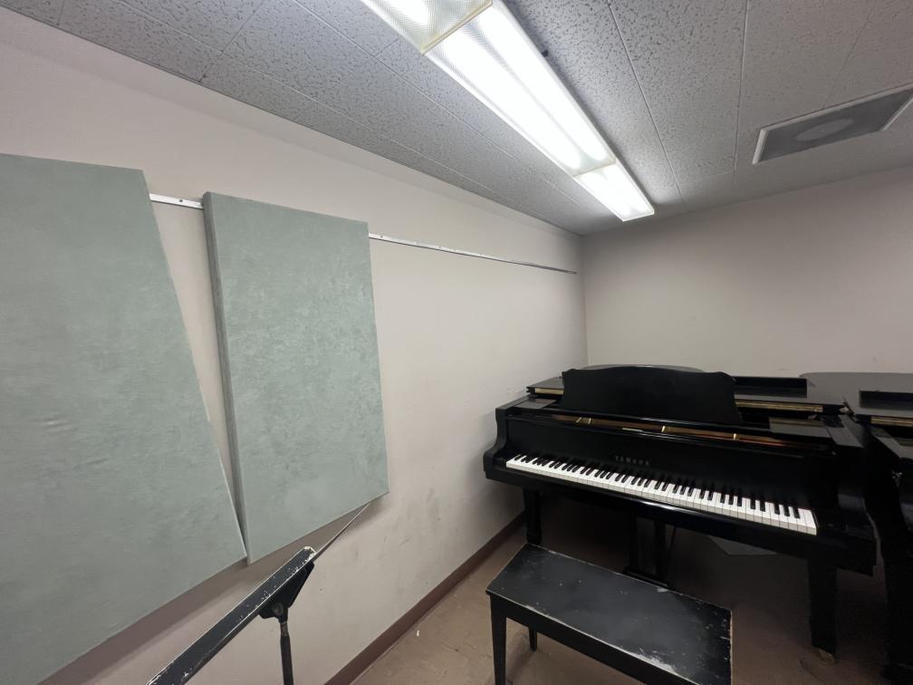
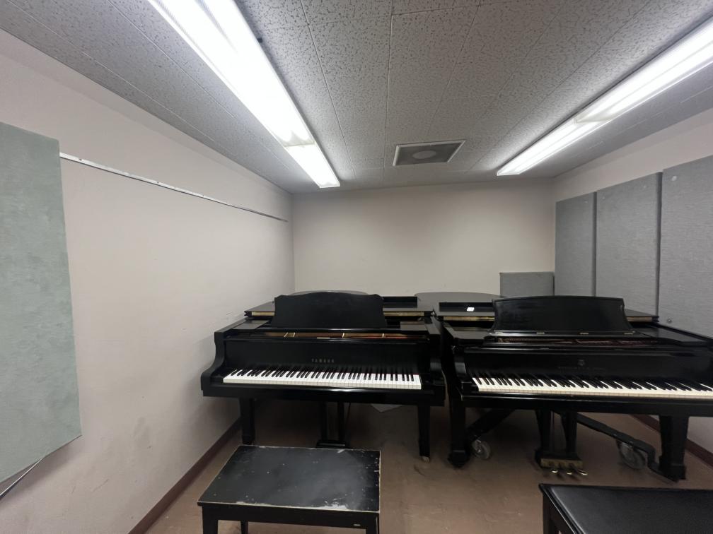
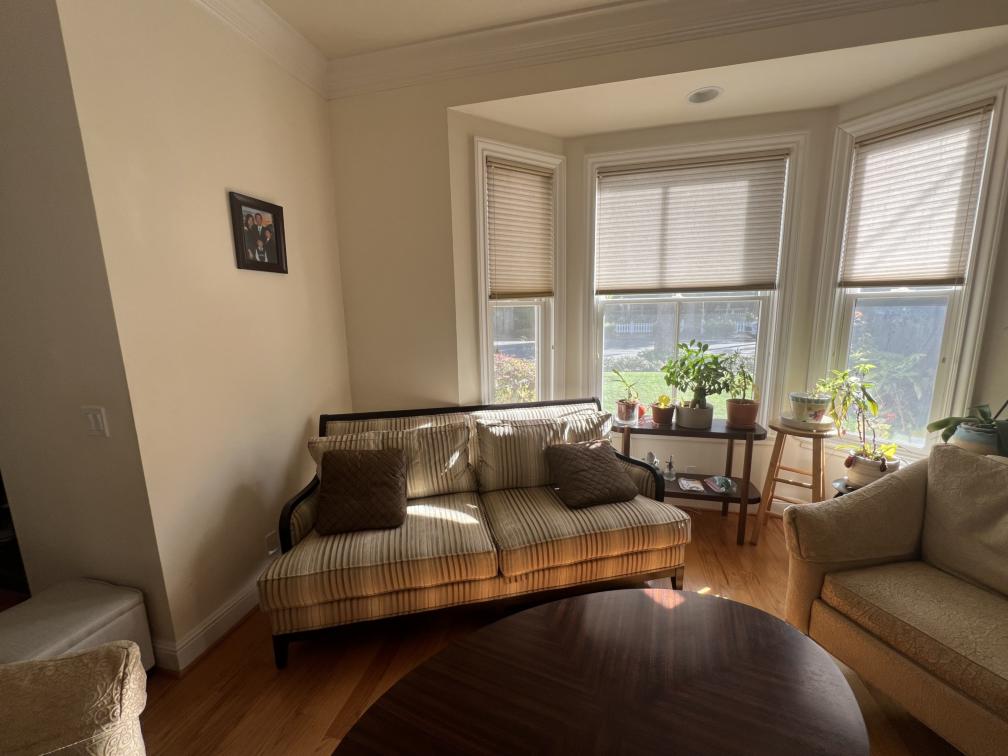
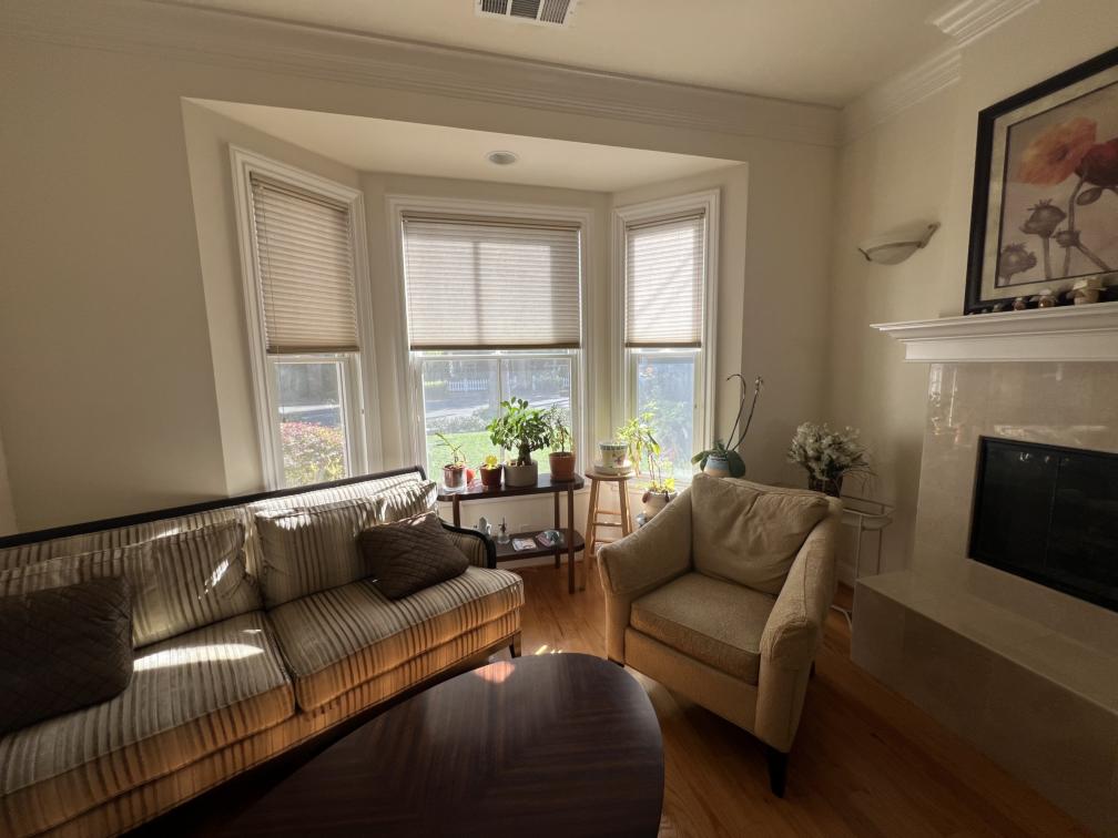
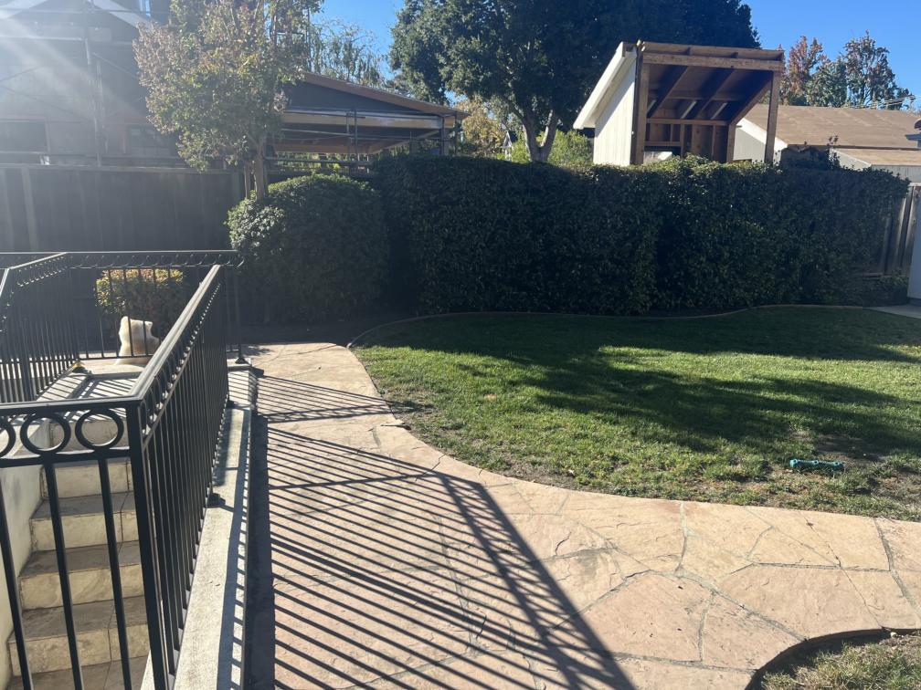
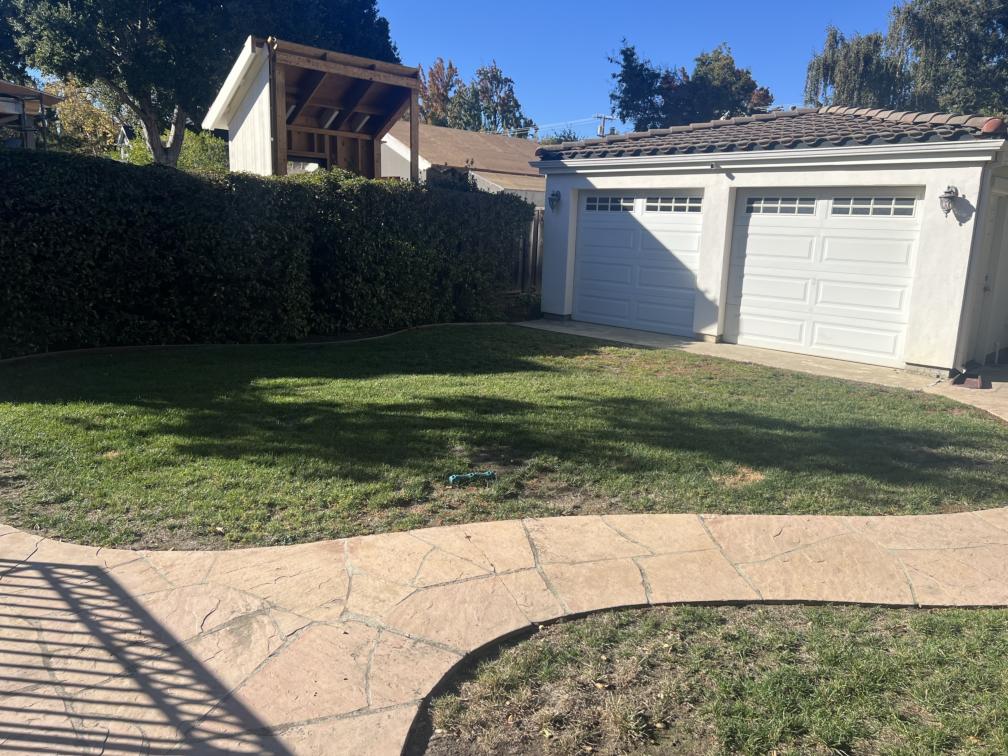
I used the following photos for this project. Corresponding pictures were taken from the same location.

|

|

|

|

|

|
To recover the homographies between images, I first hand-defined several corresponding points on several images. I then used these correspondences to derive the 8 variables in the transformation matrix. This involved rearranging the transformation equation. By using more than 4 pairs of corresponding points, we have an overdetermined system, so I used the least squares solution to the system.
To warp images into the perspective of other images, I used inverse warping and linear interpolation, similar to the previous project. I first calculated the homographies between images and applied this transformation on the corners to determine the shape of the resulting warped image. From there, I used inverse warping and interpolated pixel values from the original, unwarped image. The final image is translated to avoid having any negative pixel coordinates.
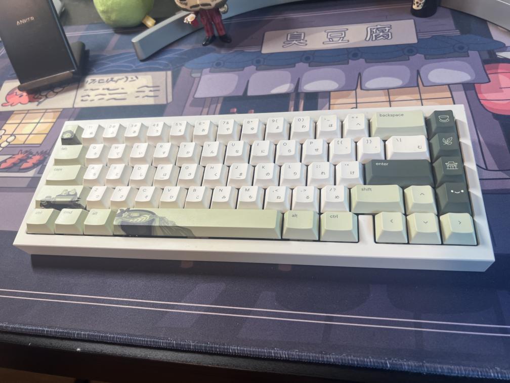
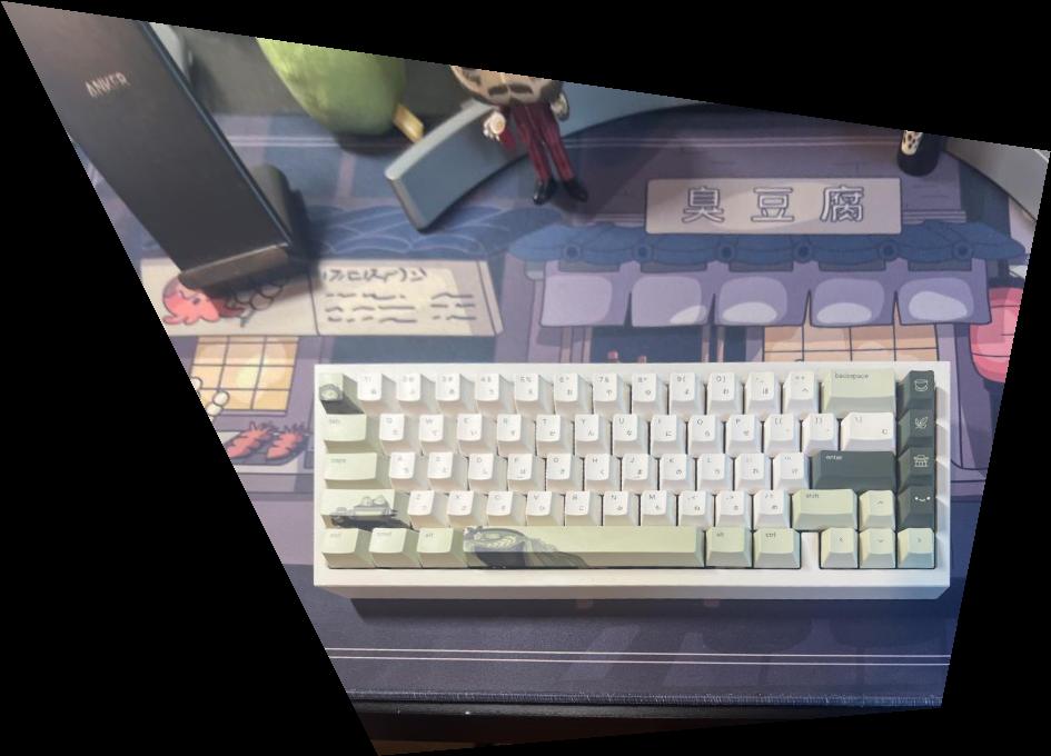
To verify the correctness of the previous two functions, I warped various images into their rectified viewing angles:
| Original | Rectified |
|---|---|
|
|
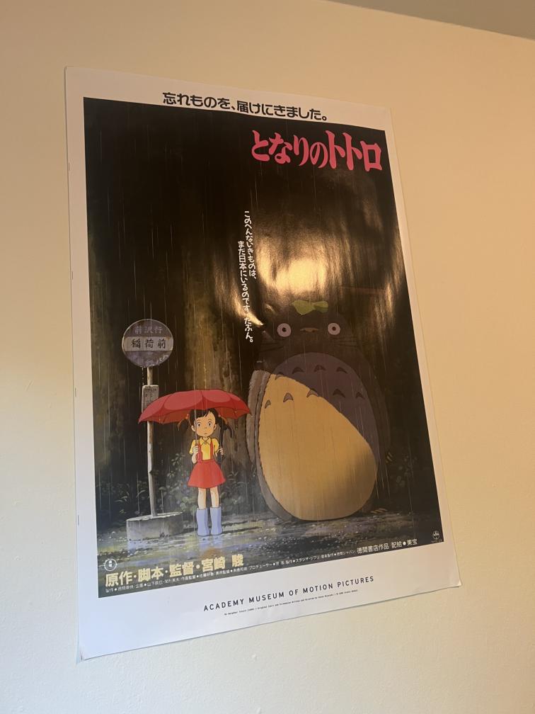
|
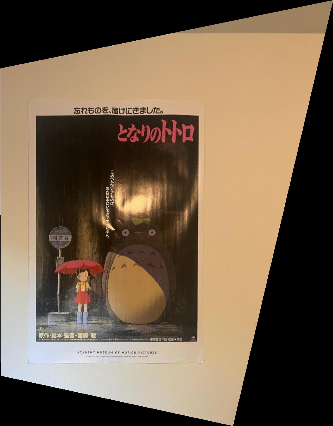
|
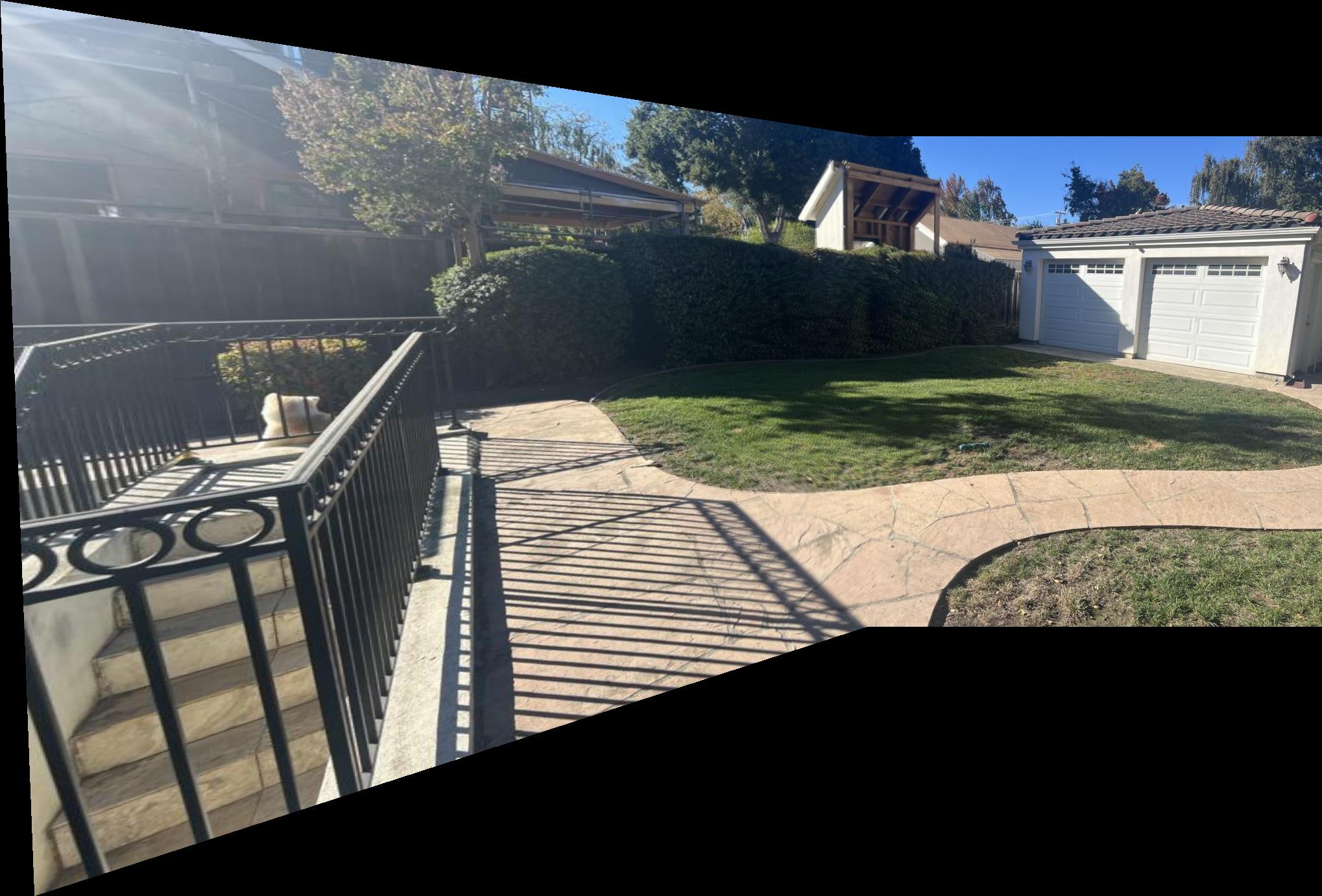
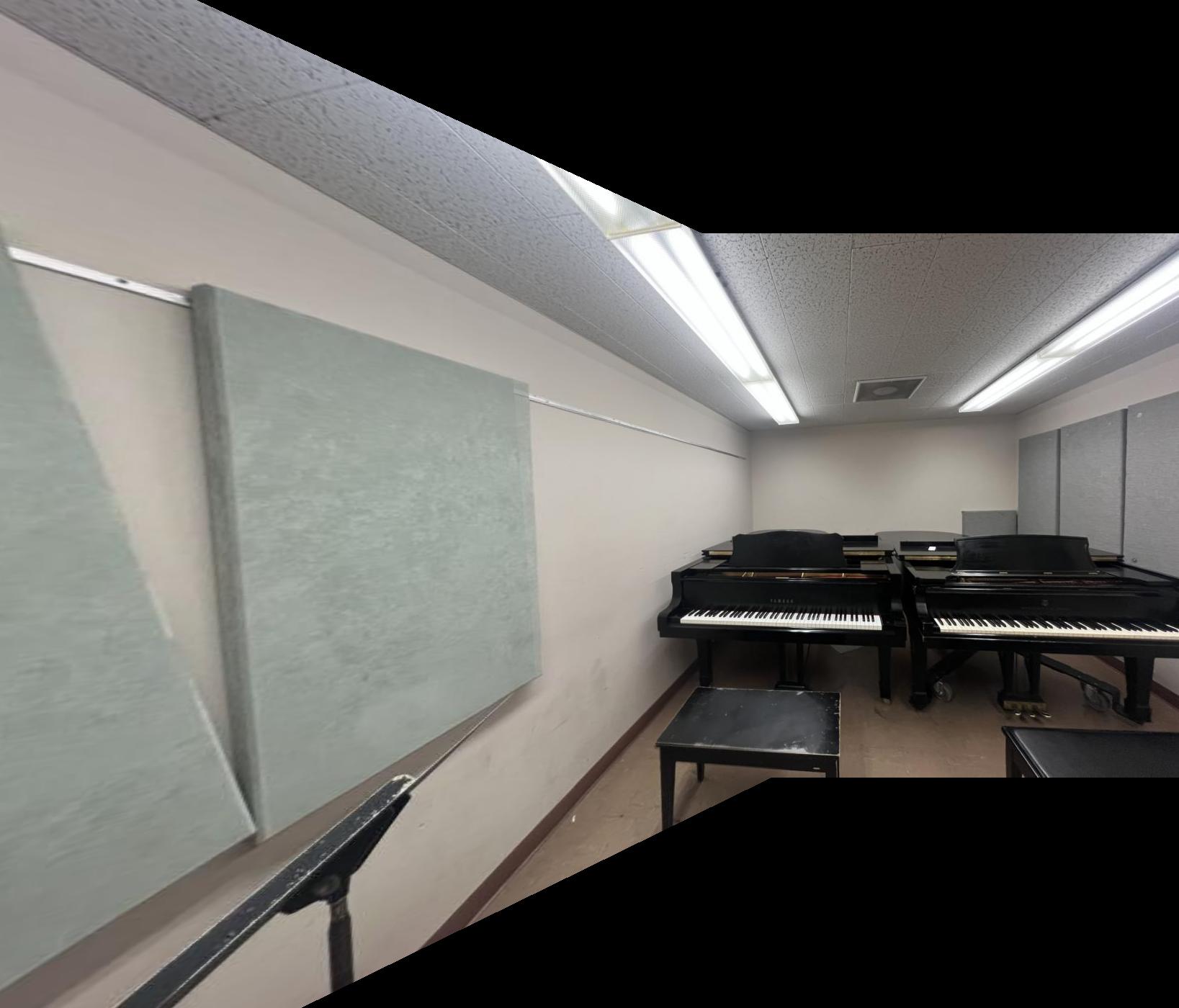
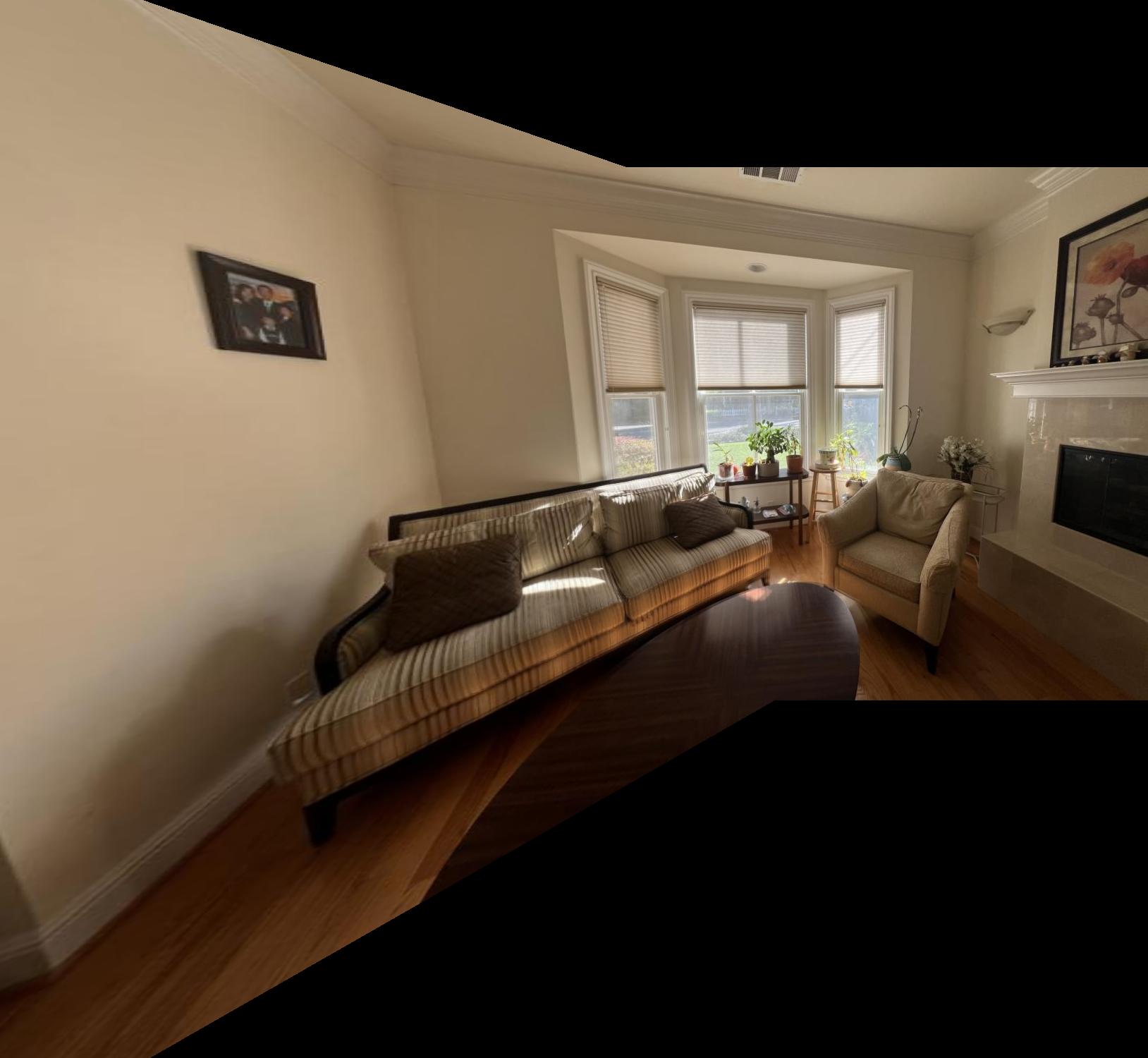
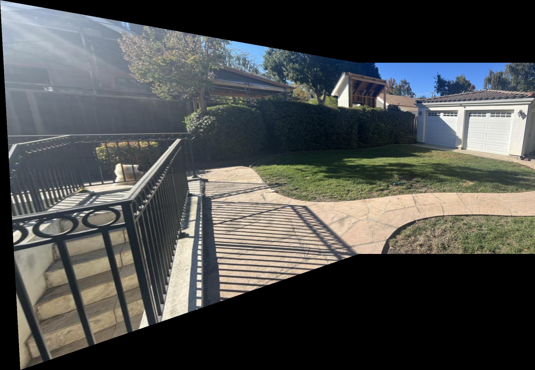
Finally, I used the warping function to generate mosaic images. To align images, I applied the translation from the image warping to the unwarped image. To blend the overlapping areas of the images, I utilized a weighted average based on the distance transform of each image. Specifically, pixels in the overlapping area are weighted by their relative distance from the non-overlapping areas of the original images. This helps to avoid any seams between images. Images that have more extreme transformations are cropped to avoid extremely large mosaics.
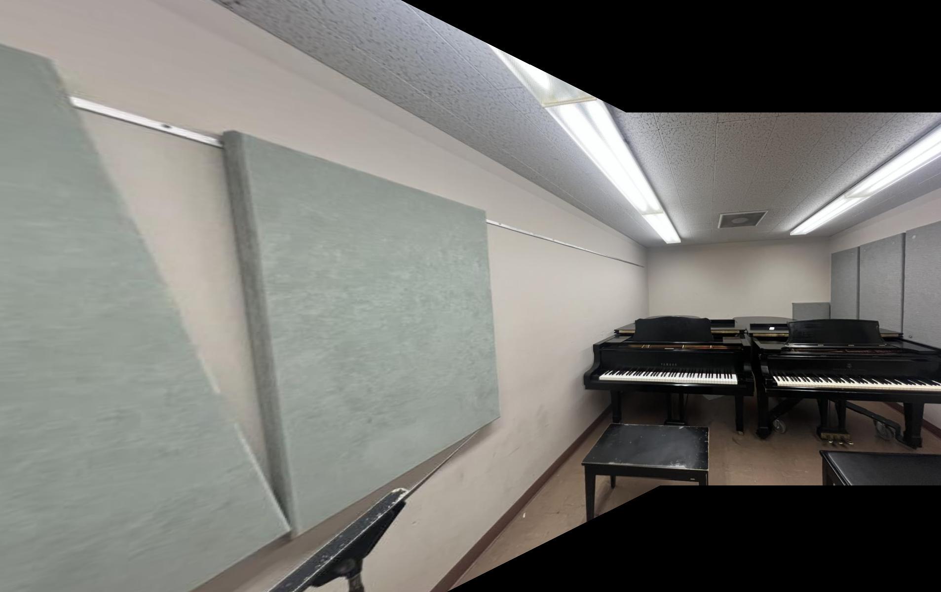
|
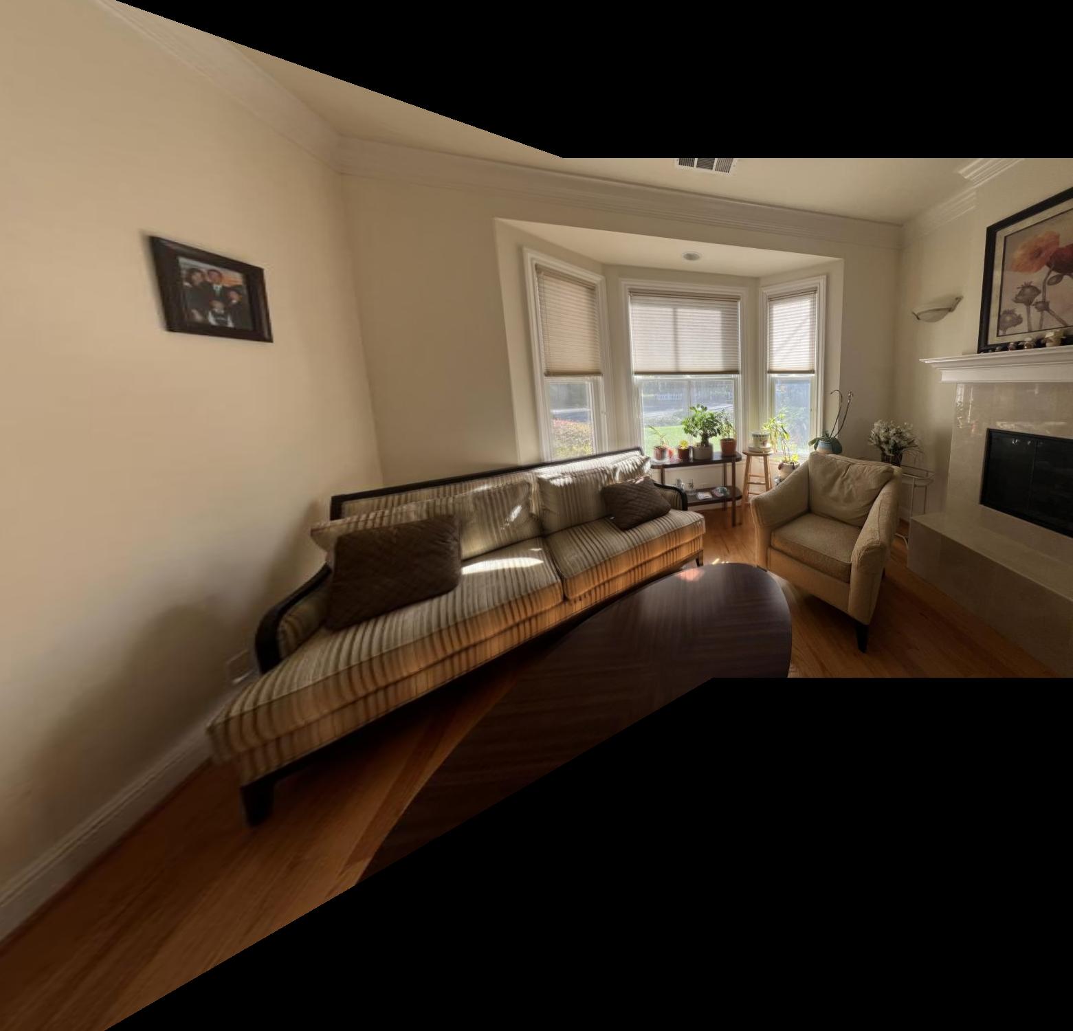
|
|
I used the provided Harris detector to find Harris corners in images. This uses a single-scale implementation and thresholds were manually selected for each image based on testing. For this image, I used a threshold of 0.03, resulting in around 2000 Harris corner points.
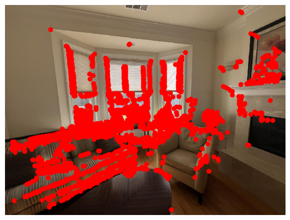
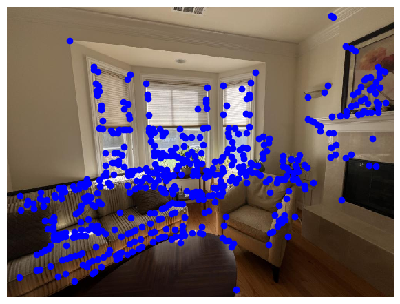
To find points with stronger corner values, I used adaptive non-maximal suppresion (ANMS) to filter the interest points. This chooses interest points by only selecting points that are local maxima within a given pixel radius. This helps to give points that are strong corners more uniformly distributed across the image. My implementation iteratively reduces this radius until a target number of points is reached or the radius is smaller than a user-defined minimum. These two parameters are selected through testing depending on the image. For the room image, ANMS chooses about 500 of the strongest interest points from the original 2000.
In order to find corresponding interest points between images, we need some descriptor for each interest point. For this project, I used an axis-aligned feature descriptor. To do this, I applied a Gaussian blur to a 40x40 pixel window around each interest point, downsampling them to 8x8 windows. These features can then be used to compare interest points across images.
Now that we have interest points and feature descriptors, we can compare interest points to find corresponding points across images to define homographies. I found matching points by using Lowe's trick. For each point in one image, I found the ratio of similarity with the 1-NN and the 2-NN. Only points with a ratio below a certain threshold are selected. The logic here is that points that are strong matches should be significantly more similar to their first nearest neighbor than the next nearest neighbor. Using a threshold of 0.4, this left 59 pairs of corresponding points for the room images:
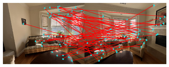
Clearly, there are still some outlier points (see the artwork in the right image, which isn't even in frame for the left image). To help mitigate the effect of these outliers, I used Random Sample Consensus (RANSAC) to define more robust homographies. This involves iteratively randomly sampling 4 pairs of corresponding points, computing a homography from these 4 correspondences, and tracking the number of inliers. The homography with the most inliers is then selected and a final homography is calculated using these inliers.
(Images are cropped to better display the stitching)
| Manual Correspondences | Automatic Correspondences |
|---|---|

|
|

|
|

|
|
I was quite careful when manually selecting corresponding points, so there is not much of a difference between the manual and automatic mosaics. This was a very interesting application of linear algebra to images and I found the techniques for mitigating outliers (ANMS, RANSAC, Lowe's trick, etc.) very satisfying.